Definition of Probability

Kolmogorov Axioms of Probability:

1. $P(\omega) = 1 , P(\phi) = 0$
2. $P(A) = 1 - P(A^c)$
3. $P(\cup_{i=1}^{\infty} A_i) = \sum_{i=1}^{\infty}P(A_i)$, where $A_i$ are mutually exclusive

What is a Random Variable a map between? $X:\omega \rightarrow R$

Random Process —> Random Event —> Random Variable —> Probability Distribution

Role of Statistics When the distribution is known but not the parameter of the distribution statistics helps you figure out the parameter

When does the classical definition of probability fail? When the set of possible outcomes are infinite.

Fischer’s Definition $\underbrace{\text{Long-run relative frequency}}_{\text{Empirical Probability}}$ is considered as definition of probability by RA Fisher

Here, $\lambda$ is the parameter of the model, and statistics is interested in finding it out. The process of searching for the $\lambda$ is called Estimation

We choose $\lambda$ values in such a way that $P(X=k)$ from the model will be very close to the empirical probability

Estimation Techniques

1. Method of Moments (Works on Toy Examples)
2. Likelihood Method (Powerful)
3. Bayesian Method (A Method in ML)

Method of Moments Assume, $X = p_{\theta}(x)$, where $\theta$ are parameters, and $p$ is either PMF\PDF based on the nature of $X$, and ${x_1, x_2, x_3, ..., x_n}$ are i.i.d samples.

Then, Sample mean: $\bar{x}$ = $\frac{\sum_{i=1}^n x_i}{n}$ = $m_1$ $m_2$ = $\frac{\sum_{i=1}^n x_i^2}{n}$, $m_3$ = $\frac{\sum_{i=1}^n x_i^3}{n}$ Sample Variance = $\frac{\sum_{i=1}^n x_i - \bar{x}}{n}$ = $m_2 - m_1^2$

Population Mean: $E[X]$ = $\sum_{x=0}^{\infty} xp_{\theta}(x)$ = $\mu_1$ $E[X^2]$ = $\sum_{x=0}^{\infty} x^2 p_{\theta}(x)$ = $\mu_2$ Population Variance: $V(X) = E[X - \mu]^2 = E[X^2] - E[X]^2$ = $\mu_2 - \mu_1^2$

The philosophy of method of moments is the sample moments should be close to the moments from the probability distribution $p_{\theta}(x)$

Basically,

and solve for $\theta$

MOM would not work when there are k unknowns but $k^{th}$ moment does not exist

What does it mean for the moment to not exist? When the function inside the summation or integral (in the case of continuous random variables) diverges for a population moment.

Probability Distribution for Continuous Random Variable

Probability Density Function $f(x)$ is a PDF such that

1. $f(x) \ge 0$
2. $\int_{R}f(x).dx = 1$

PDF is not a probability. It is a tool to $\underbrace{\text{evaluate probability}}_{P(a \lt x \lt b) = \int_a^b f(x)dx}$, whereas $\overbrace{\text{PMF}}^{0 \lt P(x) \lt 1; \sum{p(x)} = 1}$ is probability.

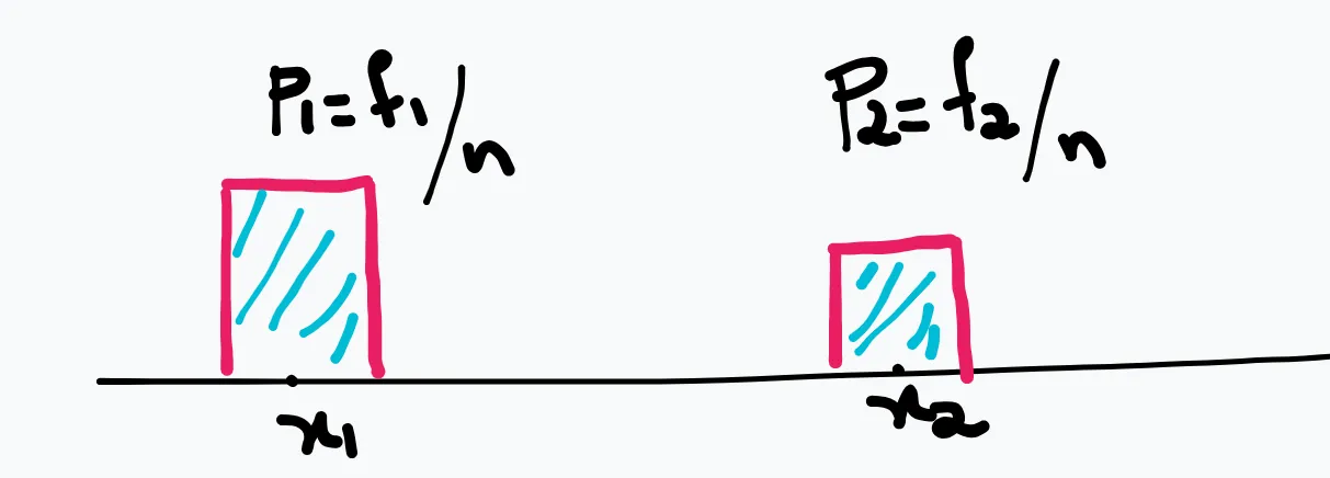
density x width = probability density = $\frac{prob}{width}$ = $\frac{p_1}{2\delta}$ = $\frac{\frac{f_1}{n}}{2\delta}$ = $\frac{\text{relative.frequency}}{width}$

a x1 x2 x3 x4 b

$P(a \lt X \lt b) = d_1(x_1 - a) + d_2(x_2 - x_1) + d_3(x_3 - x_2) + ...$ $= \sum_{i=a}^b d_i(x_i - x_{i-1})$ Approximate, $d_i = f(x_i)$ and $w_i = x_i - x_{i-1}$ As w —> 0, $\int_a^b f(x)(x_i - x_{i-1})$

If you have a function $g(x) \ge 0$ and $\int_{R} g(x) dx = a$, then $f(x) = \frac{g(x)}{a}$ is a PDF and $g(x)$ is kernel of PDF, $a$ is normalising constant.

Cumulative Distribution Function

$\int_{-\infty}^a f(x). dx = P(x \le a) = F_{x}(a)$

Moment Generating Functions

$E[g(x)] = \underbrace{\sum{g(x)P(x)}}_{\text{discrete}} = \overbrace{\int{g(x)f(x)dx}}^{\text{contiuous}}$ If X is a Random Variable with $f(x)$ as the Probability Density Function, then MGF is $E[e^{tx}] = \int{e^{tx}f(x)dx}$ (continuous) $=\sum{e^{tx}P(x)}$(discrete) $= g(t)$ $= \int{(1 + tx + tx^2/2! + ...)f(x).dx}$ (Using Taylor Series of $e^x$) $= \int f(x)dx + t\int xf(x)dx + t^2/2!\int x^2 f(x)dx + ...$ $g(t) = 1 + tE[X] + t^2/2!E[X^2] + ...$ $g^{'}(t) = E[X] + tE[X^2] + t^2/2!E[X^3] + ...$

Therefore, $g^{'}(0) = E[X]$ and $g^{''}(0) = E[X^2]$, and $V(X) = g^{''}(0) - (g^{'}(0))^2$

Why do we need the moments? I do not want to solve 4 integrations for finding the 4 properties of a distribution. I will solve 1 integration, namely $E[e^{tx}]$ and then differentiate to obtain 4 moments. Therefore, these moments help in uniquely identifying the distribution.

Raw Moments vs Central Moments? Raw Moments: Subtract “0” from X Central Moments: Subtract "$\mu$" from X

• Variance is the 2nd Central Moment and Skewness is the 3rd Central Moment Link

Cauchy Distribution $f(x) = \frac{1}{\pi} \frac{1}{1+x^2}$, where $-\infty \lt x \lt \infty$

The real moments does not exist for the distribution. It is also called as t-distribution with 1 DOF

Sampling Distribution

Population: CMI ka Students X = No. of books ordered by a student We are interested in finding $E[X] = \mu$ Define a Random Sample of size n: D = $x_1, x_2, x_3, ..., x_n$, and $\bar{x} = \frac{1}{n} \sum_{i=1}^n x_i$ Conduct this experiment many times, and plot the means. This’ll be your Sampling Distribution of the Sample Means.

Intention? Find $\mu$ The sampling distribution gives a sense of how far sample mean is away from the hypothetical true mean. It helps in quantifying the uncertainty in the data. Also helps in comparing 2 different probability estimations.

We want to figure out the sampling distribution of the sample mean from single sample Suppose $X_1, X_2, X_3, ..., X_n$ are iid $N(\mu, \sigma^2)$

We want to find $M_{\bar{X}}(t)$ $M_S(t)$ = $E[e^{ts}]$ = $E[e^{t\sum_{i=1}^n x_i}]$ = $E[\prod_{i=1}^n e^{tx_i}]$ = $\prod{(E[e^{t x_i}])}$ = $\prod{(M_{x_i}(t))}$ = $\prod{(e^{t\mu + \frac{t^2\sigma^2}{2}})}$ = $\prod{(e^{tn\mu + \frac{t^2n\sigma^2}{2}})}$ Therefore, $S \sim N(n\mu, n\sigma^2)$ We know, $\bar{X} = \frac{S}{n}$ So, $M_{\bar{X}}(t) = E[e^{t\bar{X}}] = E[e^{t\frac{S}{n}}]$ $=E[e^{\frac{t}{n}s}]$ = $\prod{(e^{\frac{t}{n} n\mu + \frac{(\frac{t}{n})^2n\sigma^2}{2}})}$ $=\prod{(e^{t\mu + \frac{t^2\sigma^2}{2n}})}$ $\bar{X} \sim N(\mu, \frac{\sigma^2}{n})$

Central Limit Theorem

$X_1, X_2, X_3, ..., X_n$ $\sim^{iid}$ $f(x)$, and $f(x)$ is an appropriate probability function such that $E[X_i] = \mu$ and $V[X_i] = \sigma^2 \lt \infty$ What is the distribution of $\bar{X}$? $M_{\bar{X}}(t) = E[e^{t\bar{X}}]$ $= \prod{E[e^{\frac{t}{n} X_i}]}$ Since, i.i.d, replace i with 1 $E[e^{\frac{t}{n} X_1}]^n$ Find MGF of $X_1$ and plug here $M_{X_1}(t) = E[e^{tX_i}] = E[1 + tX_1 + \frac{t^2X_1^2}{2} + ...]$ $= E[1 + tX_1 + \frac{t^2X_1^2}{2} + O(t)]$, since $t \sim 0$ $= 1 + t\mu + \frac{t^2E[X_1^2]}{2} + O(t^2)$ $= 1 + t\mu + \frac{t^2(\sigma^2 + \mu^2)}{2} + O(t^2)$ Therefore, $M_{\bar{X}}(t) = [M_{X_1}(\frac{t}{n})]^n$

RESULT If $X \sim N(\mu, \sigma^2)$, then $M_{X}(t) = E[e^{tX}] = e^{t\mu + \frac{t\sigma^2}{2}}$ If $X \sim N(0, \sigma^2)$, then $M_{X}(t) = E[e^{tX}] = e^{\frac{t^2\sigma^2}{2}}$ If $X \sim N(0, 1)$, then $M_{X}(t) = E[e^{tX}] = e^{\frac{t^2}{2}}$

Then, $E[\bar{X}] = E[\frac{1}{n}\sum{X_i}] = \frac{1}{n}\sum{E[X_i]} = \frac{1}{n} n\mu = \mu$ $V[\bar{X}] = V[\frac{1}{n}\sum{X_i}] = \frac{1}{n^2}\sum{V[X_i]} = \frac{1}{n^2} n\sigma^2 = \frac{\sigma^2}{n}$

Take $Z = \bar{X} - \mu$ and $M_{Z}(t) = E[e^{tZ}]$ $= E[1 + tZ + \frac{t^2Z^2}{2} + O(t^3)]$ $= 1 + tE[Z] + \frac{t^2}{2}E[Z^2] + O(t^3)$ $= 1 + 0 + \frac{t^2}{2} \frac{\sigma^2}{n} + O(t^3)$ We know, $(1 + \frac{x}{n})^n \approx e^x$, when $x$ is around 0, and $n$ —> $\infty$ Therefore, $1 + 0 + \frac{t^2}{2} \frac{\sigma^2}{n} + O(t^3) \approx e^{\frac{t^2}{2} \frac{\sigma^2}{n}}$ So, $Z = \bar{X} - \mu \approx N(0, \frac{\sigma^2}{n})$, as $n$ —> $\infty$ $\frac{\sqrt{n}(\bar{X} - \mu)}{\sigma} \approx N(0, 1)$, as $n$ —> $\infty$

Lindyberg-Levy’s CLT

Let $X_1, X_2, X_3, ..., X_n$ $\sim^{iid}$ $f(x)$ with $E[X_1] = \mu_1$ & $V(X_1) = \sigma^2 < \infty$ $Z_n = \frac{\sqrt{n}(\bar{X} - \mu)}{\sigma} \approx N(0, 1)$ as $n$ —> $\infty$

Centralise first, for quick convergence CLT fails in Cauchy, but Cauchy not seen in real-life

Bernoulli

Suppose $X_1, X_2, X_3, ..., X_n \sim^{iid} \text{Bernoulli}(p), 0 < p < 1$, where $E[X_i] = p, V[X_i] = p(1-p) < \infty$ $\bar{X} = \frac{S}{n} = \hat{p}$, where $s$ is the number of successes. 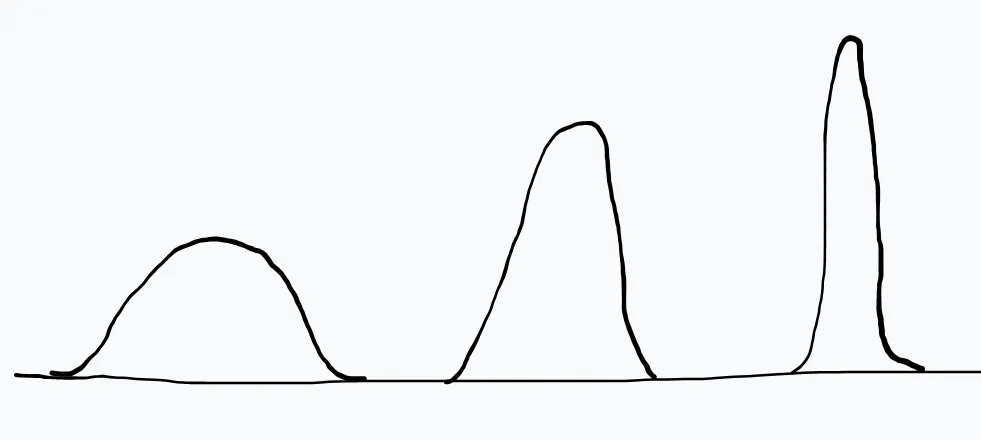$E[\hat{p}] = E[\frac{1}{n}\sum_i{X_i}] = \frac{1}{n}(np) = p$ $V[\hat{p}] = V[\frac{1}{n}\sum_i{X_i}] = \frac{1}{n^2}(np(1-p)) = \frac{p(1-p)}{n}$ By CLT, $\frac{\sqrt{n}(\hat{p} - p)}{\sqrt{p(1-p)}} \rightarrow N(0, 1)$ as $n$ —> $\infty$ For large sample, sampling distribution of sample population approximately follows Gaussian Distribution.

Gamma

Despite the fact that $\bar{X}$ of Gamma Random Variables is Gamma, the CLT still holds. Since, after a certain $n$, Gamma starts to behave as Gaussian.

Serious Criticism of TB statistical inference relying on CLT is it requires large sample size Solution? Bootstrap Statistics

Important Results

1. $Y \sim N(\mu, \sigma^2)$, then $Z = \frac{Y - \mu}{\sigma} \sim N(0, 1)$ and $Z^2 \sim \chi_{(1)}^2$
2. If $Z_1, Z_2, ..., Z_n \sim N(0, 1)$, then $S = \sum_{i=1}^n{Z_i^2} \sim \chi_{(n)}^2$
3. $X_1, X_2, ...., X_n \sim N(\mu, \sigma^2)$, then 1. $Z_n = \frac{\sqrt(n)(\bar{X} - \mu)}{\sigma} \sim N(0, 1)$ 2. $U = \frac{(n-1)s^2}{\sigma^2} \sim \chi_{(n-1)}^2$, where $s^2 = \frac{1}{n-1}\sum_{i=1}^n(x_i - \bar{x})^2$ 3. $Z_n$ & $U$ are independent of each other 4. $\frac{\sqrt{n}(\bar{x} - \mu)}{s} \sim t_{n-1}$ In part(4) of 3, if you replace $\sigma$ with estimated $\sigma$, then the distribution follows t and moves away from normal.

Statistical Inference

$\underbrace{X_1, X_2, ..., X_n}_{\text{Dataset}} \sim_{\text{iid}} F_{\theta}(x)$; $\theta$ is an unknown population parameter. Based on this dataset, make an educated guess about $\theta$

In Data Sciences, people are majorly interested in:

• $\text{I}$ : Predictive Modelling
• $\text{II}$ : Statistical Inference
  • Point Estimation / Training in ML
  • Testing of Hypotheses
  • Confidence Interval

Estimator

$T(n) = T(X_1, X_2, ..., X_n$ For example, $\hat{\theta} = \arg\max_{H} L(\theta | D) : \text{MLE}$ Any process you come up with to make an educated guess about $\theta$ $T(n) = T(X_1, X_2, ..., X_n \sim G_{\theta}(t)$, which is the CDF of sampling distribution of $T_n$

If $E[T_n] = \theta$, then we call $T_n$ as an $\underline{\text{Unbiased Estimator}}$ If $E[T_n] = \theta + \delta$ or $\theta \delta$, then we call $T_n$ as an $\underline{\text{Biased Estimator}}$

Problem

1. $\theta$ is unknown
2. We need to learn or estimate it from dataset

More Examples of Estimators

1. $T = \bar{X} = \frac{1}{n} \sum_{i=1}^n X_i$ | Sample mean is an estimator of population mean $E[X] = \mu$
2. $T = S^2 = \frac{1}{n-1} \sum_{i=1}^n (X_i - \bar{X})^2$ | Sample variance which estimates the population variance $V[X] = \sigma^2$
3. $T = S_n^2 = \frac{1}{n} \sum_{i=1}^n (X_i - \bar{X})^2$ | Sample variance which estimates the sample variance

Which is better among (2) & (3)

Competing Estimators

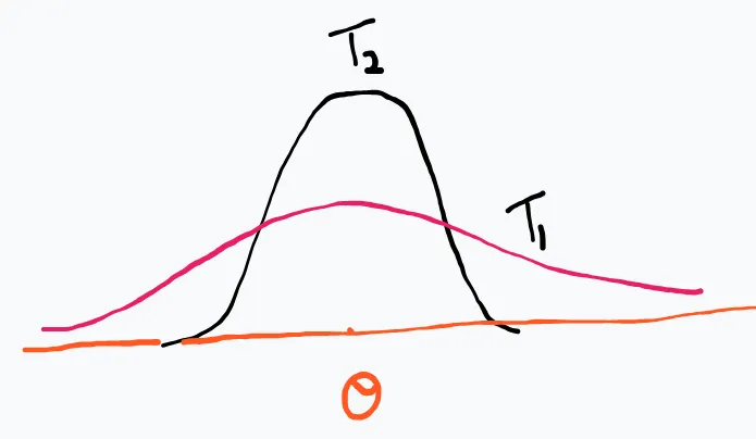
If $T_1$ and $T_2$ are two competing estimators of $\theta$, which one should we prefer? We compare their sampling distributions.

If this is the case, we clearly prefer $T_2$, as it’s more concentrated around $\theta$

We compare: $P(\theta - \delta < T_1 < \theta + \delta) < P(\theta - \delta < T_2 < \theta + \delta)$

Which corresponds to comparing the probability mass under the sampling distributions: $\int_{\theta - \delta}^{\theta + \delta} g_\theta(t_1) \, dt_1 \quad \text{vs} \quad \int_{\theta - \delta}^{\theta + \delta} h_\theta(t_2) \, dt_2$

But — we don’t know the sampling distributions of $T_1$ and $T_2$ in practice (???)

Mean Squared Error (MSE) as a Criterion

Instead, we work with something more concrete: Mean Squared Error (MSE) $\text{MSE} = \mathbb{E}[(T - \theta)^2]$ If $\text{MSE}(T_1) < \text{MSE}(T_2)$, we know $T_1$ has, on average, less error, and so we prefer $T_1$ over $T_2$.

We can decompose MSE as follows: $\mathbb{E}[(T - \theta)^2] = \mathbb{E}[(T - \mathbb{E}[T] + \mathbb{E}[T] - \theta)^2]$

Expanding this:

$\mathbb{E}[(T - \mathbb{E}[T])^2] + (\mathbb{E}[T] - \theta)^2 =Var(T)+(Bias(T))2= \text{Var}(T) + \left( \text{Bias}(T) \right)^2$ This is the bias-variance tradeoff.

Even if the bias of $T_2$ is more, if its variance is very small, we might still choose it. This tradeoff is captured in the MSE decomposition.

Concrete Example

Let $X_1, X_2, \ldots, X_n \sim \mathcal{N}(\mu, \sigma^2)$

Two estimators for population variance $\sigma^2$:

1. $S_n^2 = \frac{1}{n} \sum_{i=1}^n (X_i - \bar{X})^2$
2. $S^2 = \frac{1}{n-1} \sum_{i=1}^n (X_i - \bar{X})^2$

Consider,

$\frac{(n-1)S^2}{\sigma^2} \sim \chi^2_{n-1}$ $\mathbb{E}\left[\frac{(n-1)S^2}{\sigma^2}\right] = n - 1 \Rightarrow \mathbb{E}[S^2] = \sigma^2$

So, $S^2$ is an unbiased estimator of $\sigma^2$.

$\text{Var}\left(\frac{(n-1)S^2}{\sigma^2}\right) = 2(n - 1)\Rightarrow \text{Var}(S^2) = \frac{2\sigma^4}{n - 1}$ Since the bias is 0: $\text{MSE}(S^2) = \text{Var}(S^2) = \frac{2\sigma^4}{n - 1}$

Whereas,

$S_n^2 = \frac{1}{n} \sum_{i=1}^n (X_i - \bar{X})^2 = \frac{n - 1}{n} S^2 ⇒E[S_n^2]=E[\frac{n-1}{n}S^2]=\frac{n−1}{n}\sigma^2$

Thus, $S_n^2$ is a biased estimator of $\sigma^2$.

$\text{Var}(S_n^2) = \text{Var}\left(\frac{n - 1}{n} S^2\right) = \left(\frac{n - 1}{n}\right)^2 \text{Var}(S^2) = \left(\frac{n - 1}{n}\right)^2 \cdot \frac{2\sigma^4}{n - 1} = \frac{(n - 1)2\sigma^4}{n^2}$

$\text{MSE}(S_n^2) = \text{Var}(S_n^2) + \left(\text{Bias}(S_n^2)\right)^2 = \frac{(n - 1)2\sigma^4}{n^2} + \left(\frac{\sigma^2}{n}\right)^2 = \frac{(n - 1)2\sigma^4 + \sigma^4}{n^2} = \frac{(2n - 1)\sigma^4}{n^2}$

We want to show: $\frac{2n - 1}{n^2} < \frac{2}{n - 1}$ Multiply both sides by $n^2(n - 1)$ to eliminate denominators: $(2n - 1)(n - 1) < 2n^2$ $2n(n - 1) - (n - 1) = 2n^2 - 2n - n + 1 = 2n^2 - 3n + 1$

Compare: $2n^2 - 3n + 1 < 2n^2 \Rightarrow -3n + 1 < 0 \quad \text{(which is true for all } n > \frac{1}{3})$ ✅ So, inequality is proved.

Therefore, we found an estimator with less MSE than a minimum unbiased variance estimator.

Information

$\mathcal{D} = \{X_1, X_2, \ldots, X_n\} \overset{\text{i.i.d}}{\sim} f_\theta(x)$

• $\theta \in \mathcal{H}$: unknown parameter
• $X \in \mathbb{R}$

Likelihood Principle $\mathcal{L}(\theta \mid \mathbf{x}) = \prod_{i=1}^n f(x_i \mid \theta)$

MLE : $\hat{\theta}_{MLE} = \arg\max_{\theta \in \mathbb{H}} L(\theta | x)$

1. $\frac{\partial}{\partial\theta}log(L(\theta | x)) =^{set} 0$ to obtain where the $\theta$ maximises the likelihood function.
2. $\frac{\partial^2}{\partial\theta^2}log(L(\theta | x))$ captures how sensitive is the likelihood function for a nudge in $\theta$

Fischer’s Information

$I(\theta) = -\mathbb{E}[\frac{\partial^2}{\partial\theta^2}log(L(\theta | x))] =\mathbb{E}[\frac{\partial}{\partial\theta}log(L(\theta | x))]^2$

Example:
Let
$D = \{X_1, X_2, \ldots, X_n\} \overset{\text{iid}}{\sim} \text{Poisson}(\lambda)$

We have to figure out if $I_D(\lambda) = I_{\bar{X}}(\lambda)$: The information due to Data and whether if the information due to $\bar{X}$ is same.

If
$X_1, \ldots, X_n \overset{\text{iid}}{\sim} \text{Poisson}(\lambda)$
Then
$S = \sum_{i=1}^n X_i \sim \text{Poisson}(n\lambda)$

PMF:

So, $S$ and $\bar{X}$ are sufficient statistics of $D$ because
$I_D = I_S$

We want to calculate the information of $\bar{X}$ and show that it is sufficient.

Theorem by Fischer:
Let $T = f(S)$ be a one-one function.
Then, $T$ is also a sufficient statistic if $S$ is a sufficient statistic.

Imagine you have 100 thermometers measuring the same temperature (with Poisson noise). Each gives you one reading. But if someone tells you the total sum or average, you can figure out the temperature just as well as if you had all 100 readings. So the sum/average is all you need — it’s sufficient. And you get the same precision in your estimate (same Fisher information).

MVUE & Cramer-Rao Inequality

Suppose that $T=T(x)$ is an unbiased estimator for real-valued parametric function $\mathcal{T}(\theta)$, that is $\mathbb{E[T]} = \mathcal{T}({\theta})$ $\forall \theta \in \mathcal{H}$

Assume $\frac{d(\mathcal{T(\theta)})}{d\theta} = \mathcal{T}^{'}(\theta)$ exists and finite, Then, $V(T) \geq \frac{[\mathcal{T}^{'}(\theta)]^2}{n\mathbb{E}_{\theta}[ \frac{\partial}{\partial \theta} \log f_{\theta}(x_i)]^2} = \frac{[\mathcal{T}^{'}(\theta)]^2}{I(\theta)}$

Statistical Consistency

Population: {$X_1$, $X_2$, $X_3$, …, $X_n$} Sample: {$x_1$, $x_2$, $x_3$, …, $x_n$}

As $n \rightarrow N$, the sample(mean) should tend to population(mean)

As $n \rightarrow N$, $\bar{x} \rightarrow \mu$ {Finite Population} and $n \rightarrow \infty$, $\bar{x} \rightarrow \mu$ {To prove this, we use probability inequalities}

Markov Inequality If $X$ is a positive Random Variable, then $P(X \gt a) \lt \frac{E[X]}{a}$

Chebyshev’s Inequality

Let $X$ be any random variable with finite mean $\mu = \mathbb{E}[X]$ and finite variance $\sigma^2 = \operatorname{Var}(X) < \infty$

$\Pr\bigl(|X-\mu| \ge k\sigma\bigr) \;\le\; \frac{1}{k^{2}}$

Equivalently, $\Pr\!\bigl(-k\sigma \le (X-\mu) \le k\sigma\bigr) \;\ge\; 1-\frac{1}{k^{2}}$ $\Pr\!\bigl(\mu - k\sigma \le X \le \mu + k\sigma\bigr) \;\ge\; 1-\frac{1}{k^{2}}$

Example:
For $k = 3$ (within $3\sigma$, the probability is at least $1 - \tfrac{1}{9} = \tfrac{8}{9}$, i.e. 88.9 %.

Weak Law of Large Numbers (WLLN) Denote the sample mean by $\bar{X} \;=\; \frac{1}{n}\sum_{i=1}^{n} X_i$ Using Chebyshev on $\bar{X}$:

Hence, as $n \to \infty$, $\bar{X} \;\xrightarrow{\;\text{in probability}\;}\; \mu$

Convergence of the Sample Variance to the Population Variance

Define the (biased) sample variance $s^{2} \;=\; \frac{1}{n}\sum_{i=1}^{n}\bigl(X_i - \bar{X}\bigr)^{2}$

Our goal is to show

A Chebyshev-style bound:

Sketch of the Variance Calculation

1. Decompose each squared term

   $$\bigl(X_i - \bar{X}\bigr)^{2} \;=\; \bigl(X_i - \mu + \mu - \bar{X}\bigr)^{2} \;=\; (X_i-\mu)^{2} + (\mu-\bar{X})^{2} + 2(X_i-\mu)(\mu-\bar{X}).$$

2. Take expectations

   $$Var(s^2) = \frac{1}{n}\,\sum\!\left[(X_i-\bar{X})^{2}\right] = \frac{1}{n}\Bigl(\sigma^{2} + \operatorname{Var}(\bar{X})\Bigr) = \frac{1}{n}\Bigl(\sigma^{2} + \tfrac{\sigma^{2}}{n}\Bigr).$$

3. Result

   $$\operatorname{Var}(s^{2}) \;\propto\; \frac{1}{n}, \qquad\text{so}\qquad \operatorname{Var}(s^{2}) \;\xrightarrow{n\to\infty}\; 0.$$

Since the variance of $s^{2}$ tends to zero as $n$ grows, the probability bound above forces $s^{2}$ to converge in probability to $\sigma^{2}$.

Hypothesis Testing

$D = {X_1, X_2, ..., X_n} \sim^{\text{iid}} \text{Poisson}(\lambda)$ $H_0: \lambda \leq \lambda_{0}(=5)$ v/s $H_1: \lambda \gt \lambda_{0}(=5)$

Test 1 Test Statistic: $\bar{x}$ Reject Null Hypothesis, if $\bar{x} \gt c_1$

Test 2 Test Statistic: sample variance($s^2$) Reject $H_0$ if sample variance($s^2$) $> c_2$

Test 3 Test Statistic: Sample Median($m$) Reject $H_0$: if $m > c_3$

$\Pr(\text{Type I error}) \leq \alpha$ => $\Pr(\text{Reject Null Hypothesis, When null is true}) \leq \alpha$ ==> $\Pr(T \gt c | H_0 \text{is True}) \leq \alpha$

**Under $H_0$

1. Simulate $D^* \leftarrow {x_1^{*}, x_2^{*}, ... x_n^{*}} \sim \text{Poisson}(\lambda_0)$
2. Calculate $\bar{x}^{*}, {s^2}^{*}, m^{*}$
3. Repeat Step 1 and 2 $M$ times
4. Draw a histogram of ${x_1^{*}, x_2^{*}, ... x_n^{*}}$ | ${{s_1^2}^{*}, {s_2^2}^{*}, ... {s_n^2}^{*}}$, etc… and find c on the histogram such that the area under the curve to the right of c in the distribution is less than $\alpha$

We now would like to do intra-test comparison to figure out the test with great power

Type-II Error

$\Pr(\text{Type II error}) = \Pr(\text{Not Reject H\_0 When H\_1 is true})$

Power = 1 - Type(II)

Joint, Marginal Distributions

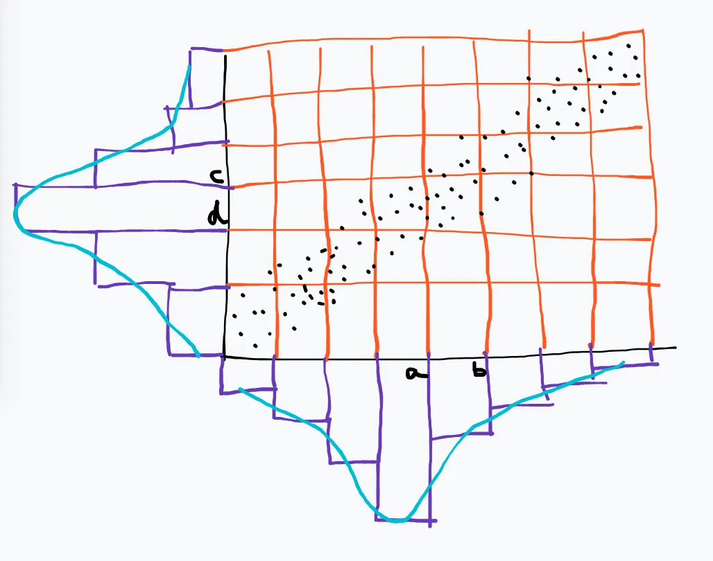
$f_i = \#(a \lt x_i \lt b$ & $c \lt y_i \lt d)$ $\tfrac{f_i}{n} = \text{rf}(a \lt x_i \lt b$ & $c \lt y_i \lt d)$ $\text{rfd} = \frac{\text{rf}}{\text{Area of the Box}}$ $\text{rfd} = \frac{\text{rf}}{(b-a)(d-c)} = \frac{\text{rf}}{\Delta{x}\Delta{y}}$ $\text{Joint Probability Density} = \frac{\text{Probability}}{\text{Area}}$

$f(x,y)$ is the joint PDF such that $(1) f(x,y) \geq 0 \forall {x,y} \in \mathbb{R}^2$ $(2)\int\int_{\mathbb{R}^2}f(x,y)dxdy=1$

$f(x)$ is the marginal PDF Distribution of $X$ where $(1) f(x) = \int_{y} f(x,y) dy$ $(2) f(y) = \int_{x}f(x,y)dx$

How do you explain the fitter line on a scatter plot from a probability perspective?

Conditional Expectation of ‘y’ given ‘x’

1. The line formed by joining the expectations of conditional distributions of $y$ given $x$ is called the regression line/function or prediction line/function
2. If Joint PDF is bi-variate or multi-variate gaussian distribution, then the resulting regression function will be a straight line

$\underbrace{\mathbb{E}[y | x]}_{\alpha + \beta x} = \int{yf(y|x)}dy$ If $(x,y)$ are assumed to be normal, then $y$ can be $\alpha + \beta x + \epsilon$ AKA straight line.

Correlation

The Degree of Linear Association

The Correlation between $x$ and $y$ depicting a upper-half of a semi-circle function will be close to zero, since correlation can only talk about the linear relationship between 2 variables.

$S_{xy} = \frac{1}{n}\sum_{i=1}^{n}(x_i - \bar{x})(y_i - \bar{y})$ (Covariance)

$r_{xy} = \frac{s_{xy}}{s_x s_y}$ (Sample Correlation) $\rho_{xy} = \frac{\mathbb{E}[X - \mathbb{E}[X]] \mathbb{E}[Y - \mathbb{E}[Y]]}{\sigma(x)\sigma(y)}$

$-1 \leq r_{xy} \leq 1$ $-1 \leq \rho_{xy} \leq 1$

Randomised Case Control Trials by RA Fischer is the currently only available way of proving causality

If you’re trying to solve OLS, then $\hat{\beta} = r\frac{s_y}{s_x}$ and $\hat{\alpha} = \bar{y} - \hat{\beta}\bar{x}$