Foundations of GAN

(Update: 29/07/2025 22:43)

This document provides a comprehensive overview of Generative Adversarial Networks (GANs), their mathematical foundations, and various implementations. It covers the motivation behind GANs, the process of generative modeling, and different types of GAN architectures including DC-GAN, Conditional GAN, and Wasserstein GAN.

This is a live document, and I will keep updating it as I implement more GANs.

Table of Contents

• Foundations of GAN
  • Motivation
  • Goal
  • Initial Plan
  • The 3-step Process of Generative Modelling
  • The Push-Forward Methods
  • Impending Questions
• Variational Divergence Minimisation
  • f-divergence
  • Algorithm for f-divergence minimization
  • Convex Conjugate
  • Realisation of VDM
  • Implementing VDM for Generative Sampling
• Generative Adversial Networks
  • GAN Architecture
  • To Train Discriminator
  • To Train Generator
  • Implementation of GAN
  • Vanilla GAN - Recap
  • GAN as Classifier-Guided Generative Sampler
• Deep-Convolutional GAN
  • Implementation of DC-GAN
• Conditional GAN
  • Implementation of Conditional GAN
• Wasserstien GAN
  • Wasserstein Metric [Optimal Transport]
  • How to do Generative Modelling with Wasserstein Metric?
  • Implementation of WGAN
• Inversion with GAN
  • Approach 1: Bi-Directional GAN
  • Latent Regression
• Handling Domain-Shift
  • Unsupervised Domain Adaptation
• Evaluation of Generative Models
  • Frechet Inception Distance
• Reference Papers

Motivation

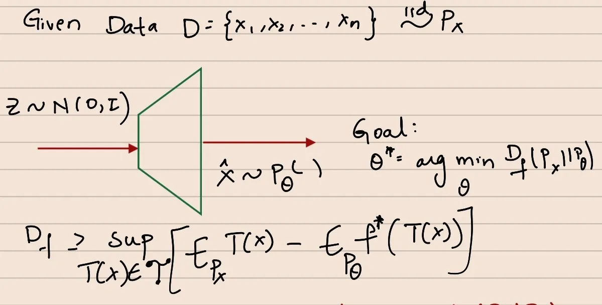
I’ve been given a sample data which is sampled i.i.d from a population. I intend to learn the parameters of the probability distribution of the population and then, sample at will.

Goal

So, I can decompose my goal into:

1. Estimate the probability distribution of the population $\mathbb{P}_{\text{data}}$
2. Learn to sample from that estimate

Initial Plan

Given, ${x_1, x_2, x_3, ..., x_n} \sim \mathbb{P}_{data}$ (unknown distribution) I’ll construct a $\mathbb{P}_{gen}$ and push $\mathbb{P}_{gen}$ towards $\mathbb{P}_{data}$

From hereon, I will refer $\mathbb{P}_{\text{data}}$ as $\mathbb{P}_{X}$ and $\mathbb{P}_{\text{gen}}$ as $\mathbb{P}_{\theta}$

Also, $\mathbb{P}$ refers to Distribution Function and $P$ refers to Probability Density Function

Assumption: Hereon, we shall solely use $P$ with the assumption that the Distribution Functions we’re dealing with have well-behaved Density Functions. [To make the calculations and math a little more easier]

Density Function is not a probability. It is a tool to evaluate probability

The 3-step Process of Generative Modelling

1. Assume a parametric family on $P_{X}$ denoted by $P_{\theta}$
   1. This $P_{\theta}$ is represented by Neural Networks
2. Define & Compute a divergence metric between the $P_{\theta}$ and $P_{X}$
   1. We don’t know $P_{\theta}$ and $P_{X}$ though?
3. Solve an optimisation problem over the parameters of $P_{\theta}$ to minimise the above divergence metric

Chalo, Assume you’ll somehow be able to compute the divergence metric between probability distributions that you don’t even know, and also optimise them, how will you begin to think about how you’ll sample from the estimated probability distribution?

The Push-Forward Methods

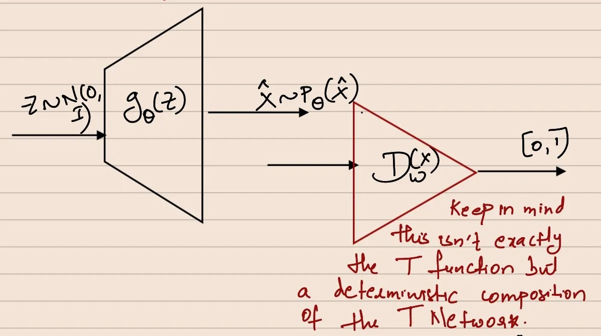
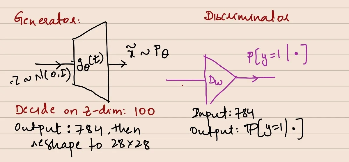
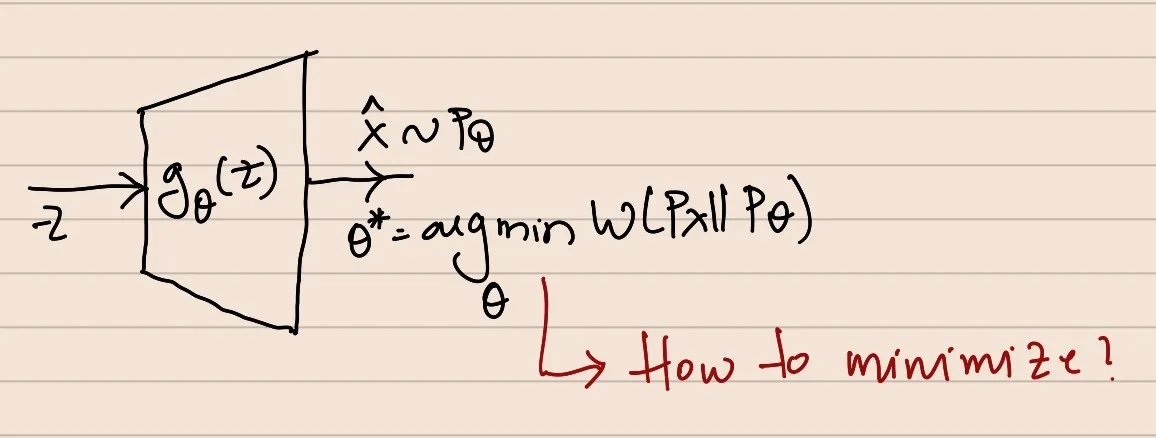
Consider some arbitrary but known distribution $Z \sim N(0, I)$ and $g_{\theta}(z): Z \rightarrow X$, then $\tilde{X} = g_{\theta}(Z)$ has a different distribution than that of $Z$. So, if you end up constructing a $g_{\theta}$ that will produce a $\tilde{X}$ that has the same distribution or close to that of $P_{X}$, we are in the game.

_Add the generator diagram here

Impending Questions

1. How to compute the divergence metric without knowing $P_{\theta}$ and $P_X$?
2. What should be the choice of the divergence metric D?
3. How to choose the $g_{\theta}(z)$, in turn, $P_{\theta}$?
4. How to solve the optimisation problem of minimising the divergence metric?

Variational Divergence Minimisation

Define DIVERGENCE between distributions

f-divergence

Given 2 probability distribution functions with the corresponding density functions denoted by $P_X$ & $P_{\theta}$, the f-divergence between them is defined as follows:

$f(u): \mathbb{R}^{+} \rightarrow \mathbb{R}$, convex, left-semi continuous, and $f(1) = 0$ $\chi:$ $\text{space on which the}$ $P_X$ $\&$ $P_{\theta}$ $\text{are supported}$

Properties of f-divergence:

1. $D_f() \geq 0$, for any choice of $f()$
2. $D_f{(P_X || P_{\theta})} = 0$, if $P_X = P_{\theta}$

Examples of f-divergence:

• KL Divergence: $f(u) = u\text{log}u$

$D_f(P_X || P_{\theta}) = \int_{\chi} P_{\theta}(x) \frac{P_X(x)}{P_{\theta}(x)} \log{(\frac{P_X(x)}{P_{\theta}(x)})} dx = \int_{\chi} P_X(x) \log{(\frac{P_X(x)}{P_{\theta}(x)})} dx = D_{KL}$

$\overbrace{D_f(P_X || P_{\theta})}^{\text{Forward KL}} \neq \underbrace{D_f(P_{\theta} || P_X)}_{\text{Reverse KL}}$ | KL-Divergence is not symmetric

Difference choices of f functions result in different divergence metric with their own properties; which necessitates the need to look at swathes of divergence metrics.

• JS Divergence: $f(u) = \frac{1}{2}(u\text{log}u - (u+1)\text{log}(\frac{u+1}{2}))$ | Used Famously in GAN
• Total Variational Distance: $f(u) = \frac{1}{2}|u-1|$

Algorithm for f-divergence minimization

Objective: Algorithm to minimise $D_f$ between $P_X$ and $P_{\theta}$, without knowing neither, but having samples from both.

Samples from $P_X$ - Dataset D Samples from $P_{\theta}$ - Outputs of $g_{\theta}(z)$ for different $z$

But, without knowing $P_{\theta}(x)$ and $P_X(x)$, solving a high-dimensional integral is infeasible.

Key Idea: Integrals involving density functions can be approximated using samples from the distribution.

The Law of Unconcisious Statistican

Suppose we wanted to compute,

where $h(x)$ is a function and $P_{X}(x)$ is the density function.

Also, suppose that we have samples drawn i.i.d from $P_X$

$x_1, x_2, x_3, ...., x_n \sim^{\text{i.i.d}} P_X$

$I = \mathbb{E}_{P_X}[h_x]$

Law of Large Numbers $\underbrace{\lim_{n \rightarrow \infty} \frac{1}{n} \sum_{i=1}^{n} h(x_i)}_{x_i \sim^{\text{i.i.d}} P_X} = E_{P_X}[h(x)]$

_If the terms of the f-divergence can be expressed in terms of expectation of functions with respect to $P_X$ and $P_{\theta}$, then one can compute and optimise them_

**Expressing $D_f$ in terms of Expectations over $P_X$ and $P_{\theta}$

$D_f(P_X || P_{\theta}) = \int_{\chi} P_{\theta}(x)f{(\frac{P_{X}(x)}{P_{\theta}(x)})}$ <--- Even though this expression looks eerily similar to the integral form of the expectation, you cannot directly rewrite that expression in terms of expectation precisely because of the arguments of f. They aren’t simply “x”, but instead are the ratio of probability density functions.

Therefore, we somehow have to decouple the ratio of PDFs from ‘f’

SLIGHT DETOUR

Convex Conjugate

If $f(u)$ is a convex function, then there exists a conjugate function

Essentially, we are lower-bounding $f(u)$ at every point t.

Properties of Conjugate

1. $f^*(t)$ is also convex
2. $[f^*(t)]^* = f(u)$ ==> $f(u) = \sup_{t \in dom (f^*)} {tu - f^*(t)}$ DETOUR DONE

$D_f(P_X || P_{\theta}) = \int_{\chi} P_{\theta}(x)f{\underbrace{(\frac{P_{X}(x)}{P_{\theta}(x)})}_{u}} \,dx = \int_{\chi} P_{\theta}(x)f(u) \,dx$ $f(u) = \sup_{t} \{{tu - f^*(t)}\}$

$D_f(P_X || P_{\theta}) = \int_{\chi} P_{\theta}(x) \sup_{t} \{{tu - f^*(t)}\} \,dx$

$D_f(P_X || P_{\theta}) = \int_{\chi} P_{\theta}(x) \sup_{t} \{{t[\frac{P_{X}(x)}{P_{\theta}(x)}] - f^*(t)}\} \,dx$

$= \sup_{T(X) \in \mathcal{T}} \int_{\chi} P_{\theta}(x) \{{T(X)[\frac{P_{X}(x)}{P_{\theta}(x)}] - f^*(T(X))}\} \,dx$

The inner optimisation problem involves $X$ & the solution for it is dependent (a function of $X$)

$\mathcal{T}: X \rightarrow dom(f^*)$ $T(X) \in \mathcal{T}$

But,

$D_f \geq \sup_{T(X) \in \mathcal{T}} \int_{\chi} P_{\theta}(x) \{{T(X)[\frac{P_{X}(x)}{P_{\theta}(x)}] - f^*(T(X))}\} \,dx$

because the space of functions $\mathcal{T}$ that we are optimising over may not contain the optimal $T^*(x)$, that is the solution for the inner optimisation problem.

Realisation of VDM

We set out to solve ---> $\theta^* = \mathop{\arg\min}_{\theta} D_f(P_X || P_{\theta})$

But we are relegated to solve $\theta^* = \mathop{\arg\min}_{\theta} [\text{lower bound on }D_f]$ and that’s the best we can do.

Calculating the supremum with respect to a class of functions $T(X) \in \mathcal{T}$ cannot be done analytically (?), since it is an optimisation procedure over a space of non-trivial functions.

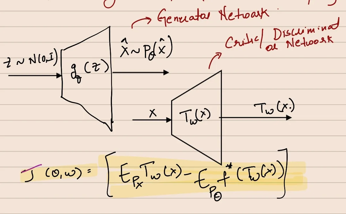
In practice, we represent $\mathcal{T}$ via neural networks: $T_w(X)$, where w are the parameters of the neural network.

With this, the objective will become:

Implementing VDM for Generative Sampling

This, essentially, is the Blueprint for Adversial Training

Any saddle point optimisation problem is also a adversial optimisation problem.

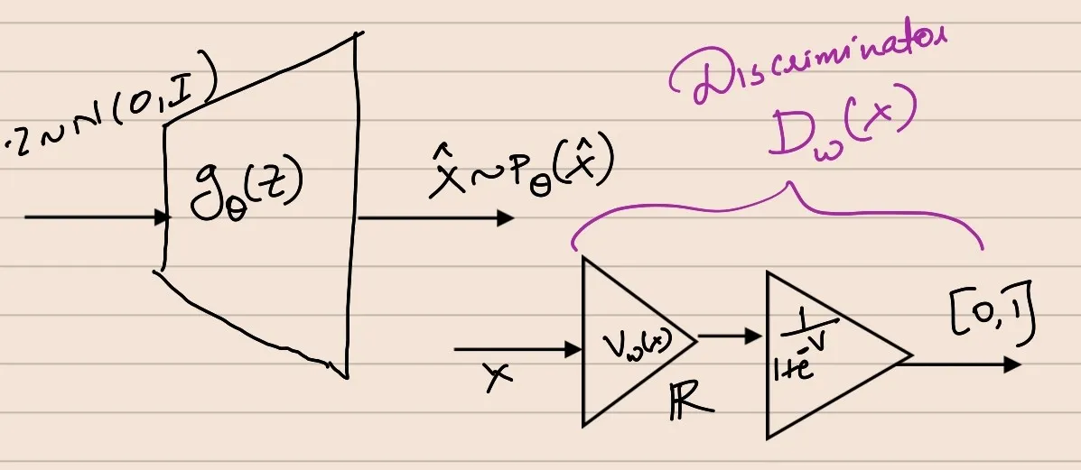
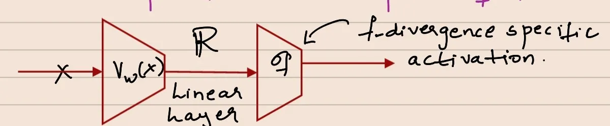
We know, by construction, $T(): X \rightarrow dom(f^*)$ ---> Depending on the choice of $f^*$, we need to tweak the T network so that the range of T network corresponds to domain of $f^*$ ---> In practice, we do this by representing $T_w(X)$ as $\sigma_f(V_w(X))$, where $\sigma_f$ is a f-divergence specific activation

$V_w(X): X \rightarrow \mathbb{R}$, $\sigma_f(v): \mathbb{R} \rightarrow dom{f^*}$

This means the T network that we’ll approximate using neural networks is represented as a composition of 2 functions.

The Discriminator as the composition of 2 functions will go here

Generative Adversial Networks

A Special Case of VDM Algorithms

The choice of f-divergence: $\overbrace{u\log u - (u+1) \log(u+1)}^{\text{Awfully similar to JS Div.}}$

$f^*(t) = -\log(1 - e^t)$ and $dom(f^*) = \mathbb{R^-}$ $\sigma_f(v) = -\log(1 + e^{-v})$

where $D_w(X) = \frac{1}{1 + e^{-V_w(X)}}$

Exercise Derive the above $J_{GAN}$ using the given f

GAN Architecture

The Generator and Discriminator go here

Assume, $\{x_1, x_2, ..., x_{B_1}\} \sim P_X$ and $\{\hat{x_1}, \hat{x_2}, ..., \hat{x_{B_2}}\} \sim P_{\theta}$

To Train Discriminator

Keep $\theta$ constant

$B_1 = \{x_1, x_2, ..., x_{B_1}\} \subset D$ | Sample $z_1, z_2, ..., z_{B_2}$ & Pass $z_1, z_2, ..., z_{B_2}$ through $g_{\theta}()$ with fixed $\theta$

$w^{t+1} \leftarrow w^{t} + \alpha_1 \nabla_{\theta}J_{GAN}(\theta, w)$

Backpropogate the gradients all the way to the inputs of the discriminator

Exercise: What is the behaviour of $D(x)$ if $P_{\theta}(x) = P_X(x)$?

To Train Generator

To update the parameters of the generator, we do not need the samples from the data.

$\theta^{t+1} \leftarrow \theta^{t} - \alpha_2 \nabla_{\theta}J_{GAN}(\theta, w)$

Typically, alternate between 1-step of Generator and 1-step of Discriminator whilst training

Implementation of GAN

class Generator(nn.Module):
  def __init__(self, noise_dim, img_dim):
    super(Generator, self).__init__()
    self.model = nn.Sequential(
        nn.Linear(noise_dim, 256),
        nn.ReLU(True),
        nn.Linear(256, 512),
        nn.ReLU(True),
        nn.Linear(512, 1024),
        nn.ReLU(True),
        nn.Linear(1024, img_dim),
        nn.Tanh() # Because we normalized images to [-1, 1]
    )

  def forward(self, z):
    return self.model(z)

class Discriminator(nn.Module):
  def __init__(self, img_dim):
    super(Discriminator, self).__init__()
    self.model = nn.Sequential(
        nn.Linear(img_dim, 512),
        nn.LeakyReLU(0.2, inplace=True),
        nn.Linear(512, 256),
        nn.LeakyReLU(0.2, inplace=True),
        nn.Linear(256, 1),
        nn.Sigmoid() # Outputs probability between 0 and 1
    )

  def forward(self, img):
    return self.model(img)

def train_gan(train_loader, num_epochs:
  fixed_noise = torch.randn(64, noise_dim).to(device)

  for epoch in range(num_epochs):
    for batch_idx, (real, _) in enumerate(train_loader):
      batch_size = real.size(0)
      real = real.view(batch_size, -1).to(device)

      ### Create Real and Fake Labels
      real_labels = torch.ones(batch_size, 1).to(device)
      fake_labels = torch.zeros(batch_size, 1).to(device)

      ### ==================================
      ### Train Discriminator: max log(D(x)) + log(1 - D(G(z)))
      ### ==================================

      # Real Images
      outputs = discriminator(real)
      d_loss_real = criterion(outputs, real_labels)
      real_score = outputs

      # Fake Images
      z = torch.randn(batch_size, noise_dim).to(device)
      fake = generator(z)
      outputs = discriminator(fake.detach())
      d_loss_fake = criterion(outputs, fake_labels)
      fake_score = outputs

      # Total Loss
      d_loss = d_loss_real + d_loss_fake

      # Backprop
      d_optimizer.zero_grad()
      d_loss.backward()
      d_optimizer.step()

      ### ================================
      ### Train Generator: min log(1 - D(G(z))) <-> max log(D(G(z))
      ### ================================
      # Generate fake images again
      z = torch.randn(batch_size, noise_dim).to(device)
      fake = generator(z)
      outputs = discriminator(fake)

      g_loss = criterion(outputs, real_labels) # trick discriminator

      # Backprop
      generator.zero_grad()
      g_loss.backward()
      g_optimizer.step()

      if (epoch + 1) % 10 == 0:
		print(f"Epoch [{epoch+1}/{num_epochs}], D_loss: {d_loss.item():.4f}, G_loss {g_loss.item():.4f}")
		show_generated_images(epoch+1, generator, fixed_noise)

Vanilla GAN - Recap

Input: D = $\{x_1, x_2, ..., x_n\} \sim^{\text{i.i.d}} P_X$ Data: $\text{MNIST}_{28\texttimes28}$

Loss Function

Approximate expectation using Sample Mean and use Batches

$x_1, x_2, ..., x_{B_1} \sim^{\text{i.i.d}} P_x$ $\hat{x_1}, \hat{x_2}, ..., \hat{x_{B_2}} \sim^{\text{i.i.d}} P_{\theta}$

$z_1, z_2, ..., z_{B_2} \sim^{\text{i.i.d}} N(0, I)$

Discriminator N/W:

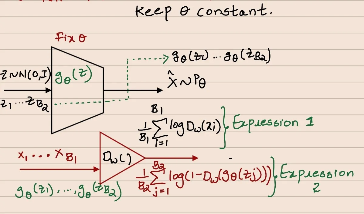
While training the discriminator the parameters of the generator network are kept constant.

1. Sample $z_1, z_2, ..., z_{B_2} \sim^{\text{i.i.d}} N(0, I)$
2. Pass them through $g_{\theta}(z)$ to obtain $g_{\theta}(z_1), g_{\theta}(z_2), ..., g_{\theta}(z_{B_2})$
3. Pass these through $D_w(.)$ and obtain the $2nd$ term in loss
4. Get $x_1, x_2, ..., x_{B_1} \sim P_x$
5. Pass these through $D_w(.)$ and get the 1st term in loss
6. TOTAL LOSS = TERM 1 + TERM 2

This is how the gradient ascent is implemented for the discriminator network.

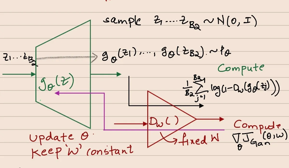
Generator N/W:

While training the generator the parameters of the discriminator network are kept constant.

GAN as Classifier-Guided Generative Sampler

$D = \{x_1, x_2, ..., x_n\} \sim^{\text{i.i.d}} P_X$

Goal: $P_{\theta}(\hat{x})$ to be close to $P_X$

Suppose there’s a binary classifier,

$D_w(X)$ is a binary classifier between the samples of $P_X$ and $P_{\theta}$

Question: Can $D_w(X)$ be used to make $P_X$ and $P_{\theta}$ closer? Answer: Yes. Tweak $\theta$ till the classifier fails to distinguish between the samples of $P_X$ and $P_{\theta}$

However, Failure of the classifier need not imply $P_X = P_{\theta}$ (A counter example supporting this statement can be easily formed)

Solution: Keep altering the classifier along with the data (pretty intuitive)

Natural Question: What if the data clusters just cycles around 2 positions? We may get stuck!!!

This is Possible. It’s called MODE COLLAPSE, a failure mode in GANs

Formulation

Suppose, $D_{w}: X \rightarrow [0, 1]$ Let $D_w(X)$ represent the likelihood of sample $X$ coming from $P_X$

The objective is to maximise the log-likelihood of $X$ coming from $P_X$

Maximising the likelihood of $X \sim P_X$

Classifier should also maximise the likelihood of $\hat{X}$ not coming from $P_X$, when $\hat{X} \sim P_{\theta}$

Maximising the likelihood of $\hat{X} \not\sim P_X$

The Combined Objective For Classifier Training

Same as the loss-function we’ve obtained in the VDM.

The Objective for The Generator

It’s job is to make the classifier “fail”

Invert the optimisation for the classifier

This classifier-guided interpretation of GAN is not generalizable across other f-divergences. Because, there’s no guarantee that the T function we use to bound the f-div has the interpretation that T-function is a classifier. Only with this particular choice of f-divergence do we have that interpretation.

Deep-Convolutional GAN

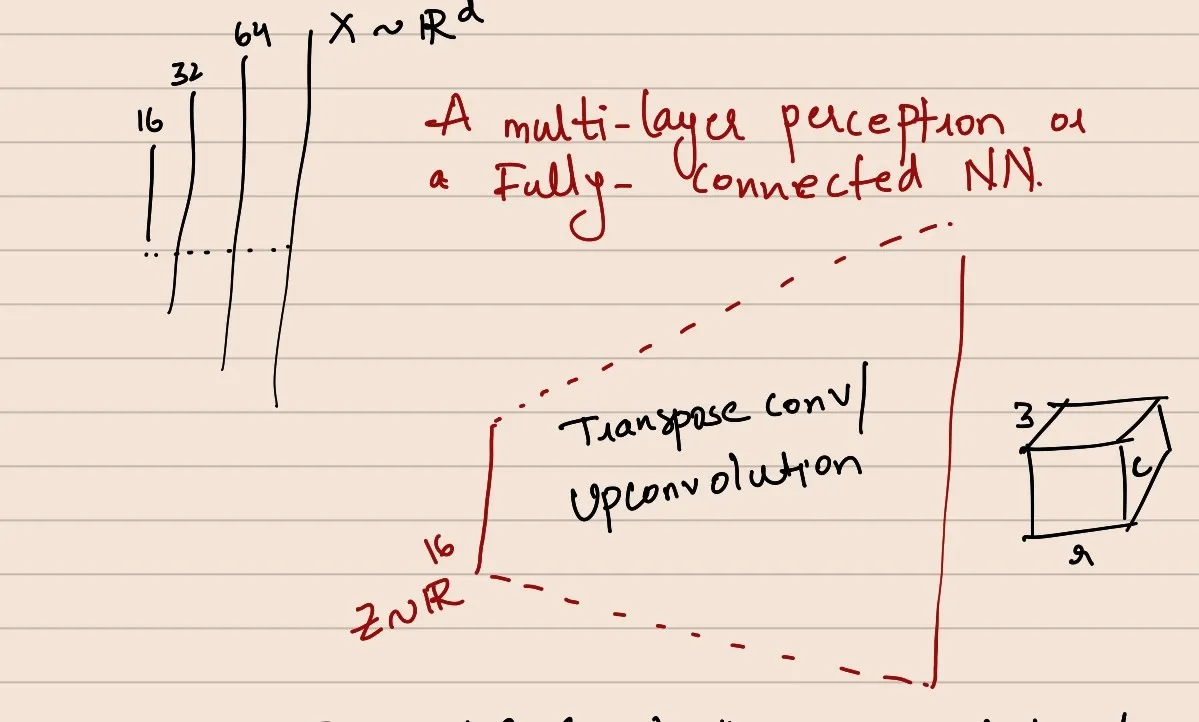
Typically, in a GAN, $\mathcal{Z} \in \mathbb{R}^{k}, X \in \mathbb{R}^d, k << d$

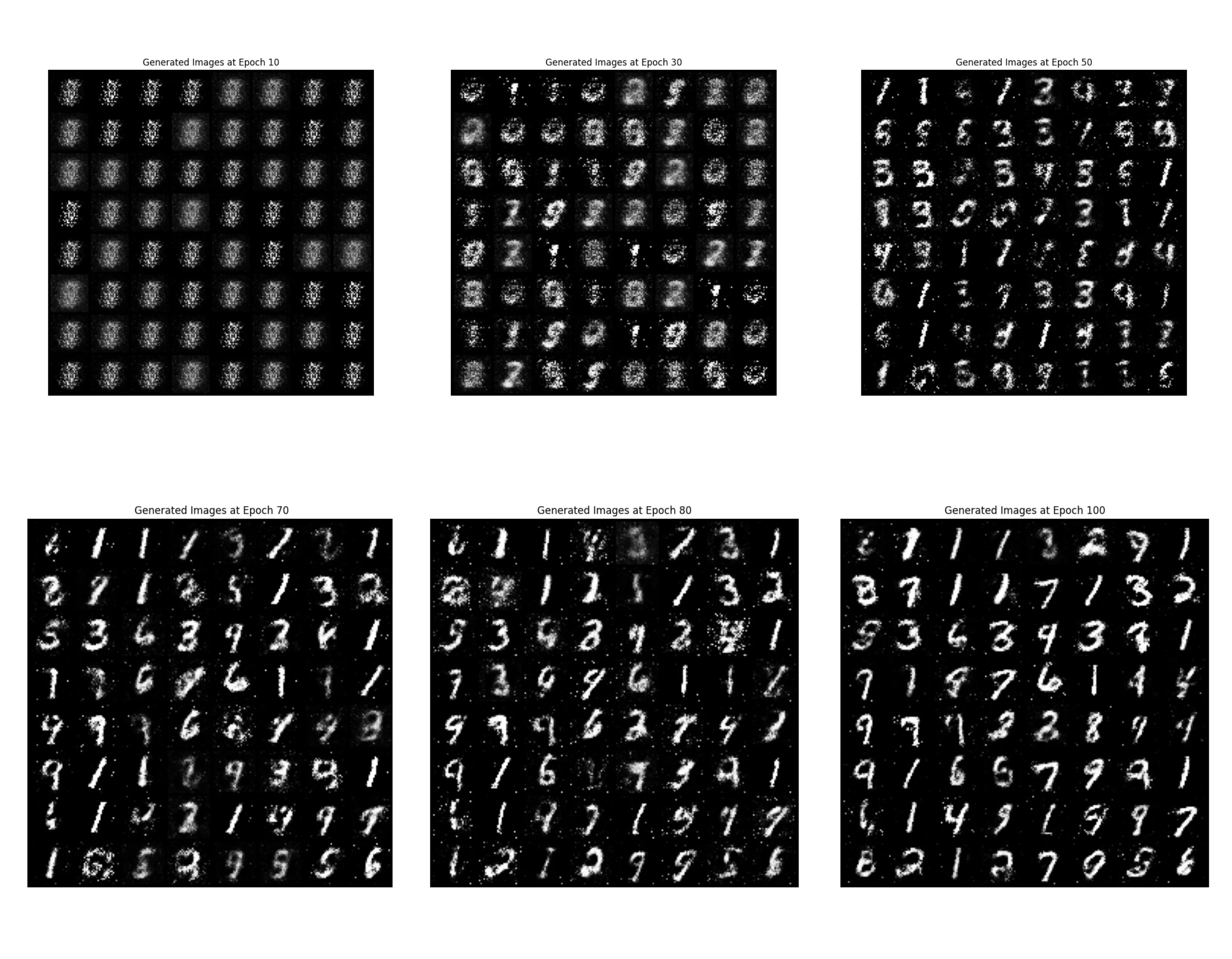
In a DC-GAN, Upconvolution (or transpose convolutional) layers are used in the generator. In DC-GAN, data is images

Implementation of DC-GAN

Conditional GAN

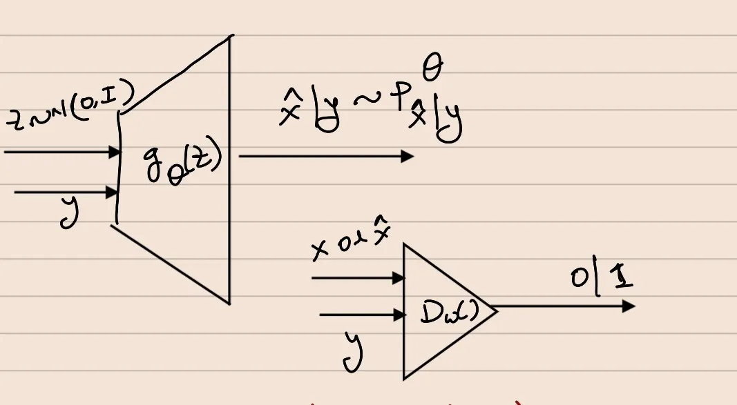
Data D: $\{(x_1, y_1), (x_2, y_2), ..., (x_n, y_n)\} \sim^{\text{i.i.d}} P_{XY}$ Example: $X$ : Images, $Y$ : class-label / textual embedding

Objective: Sample from conditional distribution $P_{X | Y}$ instead of $P_X$ (Naive GAN)

Solution: Estimate $P_{X | Y}$ and make $P_{\theta}$ approach $P_{X | Y}$ $\forall y$

Modify the generator & discriminator to operate on the samples of conditional distribution.

Implementation of Conditional GAN

Wasserstien GAN

Motivation for the Need

1. The saddle point optimisation problem is difficult
2. Any f-divergence minimisation leads to unstable training

Question: What makes GAN training difficult and unstable?

Manifold Hypothesis

The data we observe in the wild reside in a very low-dimensional manifold in the ambient space $(\mathbb{R}^d)$

Example ${\text{pixel}} \begin{array} {|r|r|} \hline 0 & 1 & 1 & 0 & 0 \\ \hline 1 & & & & \\ \hline & & & & \\ \hline & & & & \\ \hline & & & & \\ \hline \end{array}$ Consider this 5 x 5 image with $P_{ij} = 1$ if toss is heads & vice-versa. The likelihood that an image generated by the above process resembles a real-world image is very low.

Therefore, it can be posited that real data exists on a lower dimensional manifolds.

Consequently, the supports of $P_X$ and $P_{\theta}$ will not be aligned with a very high probability.

It can be shown that a Perfect Discriminator can be learned when the supports of $P_X$ and $P_{\theta}$ are not aligned.

==> The GAN Training Saturates: Perfect Discriminator Theorem For a perfect discriminator, the gradients flowing to generator nullify. Alternatively, it can be said that the lower bound on the loss is not tight, therefore minimising it would not make sense.

When we have a perfect discriminator ---> the $D_f(P_x || P_{\theta})$ becomes independent of ${\theta}$
---> this causes saturation ---> Since, the gradients won’t flow to the generator, you wouldn’t be able to tweak the $\theta$ to make the generated data align with real data, effectively.

1 Empirical Solution is to not train them equally. 1 Principled Solution is to use a softer divergence metric that does not saturate when the manifolds of the supports of $P_X$ and $P_{\theta}$ do not align.

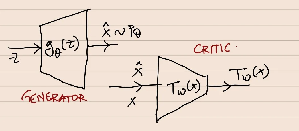
Wasserstein Metric [Optimal Transport]

Idea: We will show that the Wasserstein metric will not saturate and won’t become independent of generator’s metrics, despite the manifold of supports not aligning.

Given 2 distributions, $P_X$ & $P_{\theta}$

$\lambda: \text{joint distribution between } P_X, P_{\hat{X}}$ $\Pi(X, \hat{X})$: All possible joint distributions such that $\int_x \Pi(x, \hat{x}) \,dx = P_{\hat{x}}$ & $\int_{\hat{x}} \Pi(x, \hat{x}) \,d\hat{x} = P_{x}$

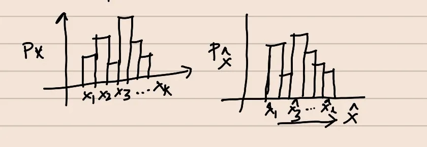
Example: Suppose $P_X$ and $P_{\hat{X}}$ are two 1-d discrete PMF.

The mass in $P_X$ can be redistributed such that $P_X$ transforms into $P_{\hat{X}}$ A redistribution scheme can be represented as a joint distribution between $P_X$ and $P_{\hat{X}}$

_Joint Distribution between $P_X$ and $P_{\hat{X}}$_

Every redistribution scheme is a joint distribution and it is called a transport plan.

Next Goal:

Quantify the effort involved in a transport plan.

Suppose some mass is moved from $X$ and $\hat{X}$, then $||X - \hat{X}||_2: \text{Distance of the Movement of Mass}$

Any work done in a transport plan:

_Why are we doing this? We are in search of metric that tells us the work needed to move one distribution to another.

Given that multiple transport plans (Joint Distributions) exist between $X$ and $\hat{X}$, which of them would correspond to least amount of work done?

This corresponds to the transport plan leading to the least amount of work done.

The closer the $P_X$ and $P_{\hat{X}}$ are the lesser the amount of work needed by the transport plan.

Wassertstein’s Metric between 2 distributions $P_X$ and $P_{\hat{X}}$ is given by:

Fact | Take-Home Message: Wasserstein’s Metric does not saturate unlike f-divergences, when supports of $P_X$ and $P_{\theta}$ does not overlap

How to do Generative Modelling with Wasserstein Metric?

$\theta^* = \mathop{\arg \min}_{\theta} W(P_X || P_{\theta})$ ---> How to minimise? ---> Cue the Kantrovich-Rubenstein Duality

==> A function is $\text{1-Lipschitz}$ if it’s rate of change is bounded by 1.

AKA: Bounded Derivatives

The above objective is very similar to GANs. Thus, the above method of minimising the wasserstein metric is called W-GAN.

$T_w(X)$ has to be made $\text{1-Lipschitz}$ ---> How to achieve this is a research topic in itself ---> 1 Practical way to achieve this ---> Normalise the weights of $T_w$ such that $||w||_2 = 1$ after each gradient step.

CONCLUSION: It is observed that training W-GAN is more stable compared to that of Naive GAN.

Implementation of WGAN

Inversion with GAN

A trained GAN is a function $Z \rightarrow X$. Suppose one is interested in inversion of the above function,i.e, given $x_i \sim P_x$, find the corresponding $Z$ ---> $z_i: g_{\theta}(z_i) = x_i$

Question: How to modify a GAN such that the inverse is possible?

First off, why is it worthy of our attention?

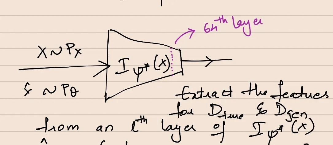
1. Feature Extraction: Given a dataset obtain GAN-inverted vectors and use them as features for data. They, then, can be used for downstream tasks.
2. Data Manipulation & Editing: Suppose $x_i \sim P_x$ needs to be edited. First, obtain $x_i = g_{\theta}^*(z_i)$ via inversion. Then, $z_{\text{edit}} = f_{\text{edit}}(z_i)$ & $x_{\text{edit}} = g_{\theta}^*(z_{\text{edit}})$

Approach 1: Bi-Directional GAN

In a Naive-GAN, $g_{\theta}(z):Z \rightarrow X$ $D_w(x): X \rightarrow [0, 1]$

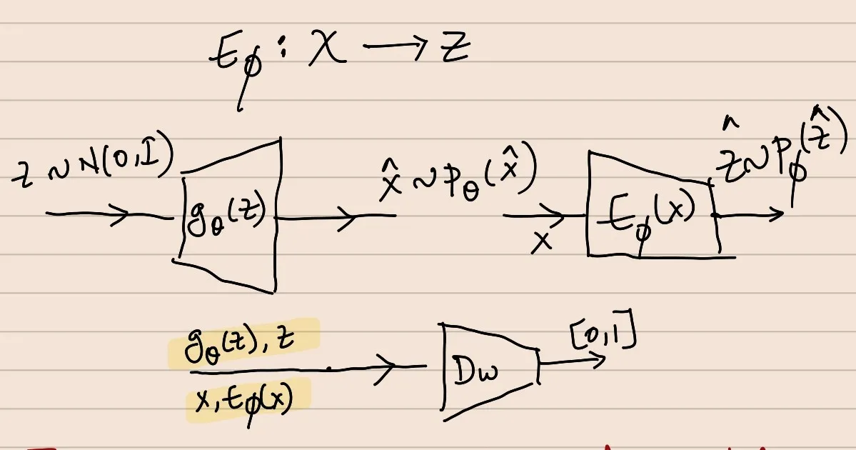
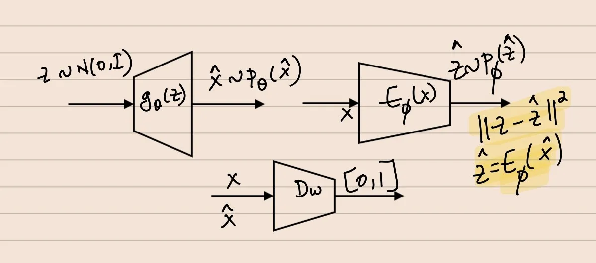
In Bi-GAN, in addition to $g_{\theta}(z)$ & $D_w(x)$, there is another function called the Encoder or the Invertor network ---> $E_{\phi}: \chi \rightarrow Z$

In Bi-GAN, the $D_w()$ is designed to classify between the data tuples of the form $[X,E_{\phi}(X)] \text{ and } [g_{\theta}(Z), Z]$, where $X \sim P_X$, $E_{\phi}(X) \sim P_{\phi}(\hat{Z}), Z \sim N(0, I), g_{\theta}(Z) \sim P_{\theta}$

In a Naive-GAN, $D_w()$ classifies between $X \text{ and } g\_{\theta}(Z)$

Objective Function for BiGAN

Once a Bi-GAN is trained, the generator network $g_{\theta}^*(z)$ is used for generation & $E_{\phi}^*(x)$ is used for inversion.

It can be shown that the optima of $L_{\text{Bi-GAN}}$ is achieved when $P_{\hat{Z}X} = P_{Z\hat{X}}$, where $P*{\hat{Z}X} = \int_xP_x\int*{\hat{z}}P*{\phi}(\hat{z} | x).d{\hat{z}}.dx$ $P*{Z\hat{X}} = \int*zP_z\int*{\hat{x}}P\_{\theta}(\hat{x} | z).d{\hat{x}}.dz$

Implementation of BiGAN

Latent Regression

Handling Domain-Shift

You made a classifier in Delhi. Want to use in Boston. How to make it robust to that change? By extracting domain-invariant features

Suppose we have data from a distribution,

$D_S$: Source Distribution

Task: Classification, Estimate $P_S(y | x)$

During test-time, data comes from a different distribution. $D_T$ that is different from $D_S$

Classifiers / Regressors trained on $D_S$ would fail on $D_T$ [PACS Dataset]

Unsupervised Domain Adaptation

Given D_S = \{(x_i, y_i)\}_{i=1}^n \mathop{\sim}^{\text{i.i.d}} P_S$$$$D_T = \{(\hat{x_j})\}_{j=1}^m \mathop{\sim}^{\text{i.i.d}} P_T$$$$P_S \neq P_T (Domain-Shift)

Objective: Given $D_S$ & $D_T$, learn features/classifier such that it performs well on both source and target data

Solution: Domain Adversial Networks

$\phi: \chi \rightarrow F$ | $\phi(x) = f_S$ & $\phi(\hat{x}) = f_T$ $f_S \sim P_{f_S}$ $f_T \sim P_{f_T}$

The $\phi$-network has 2 objectives

1. Adversial Objective
2. Classification Objective

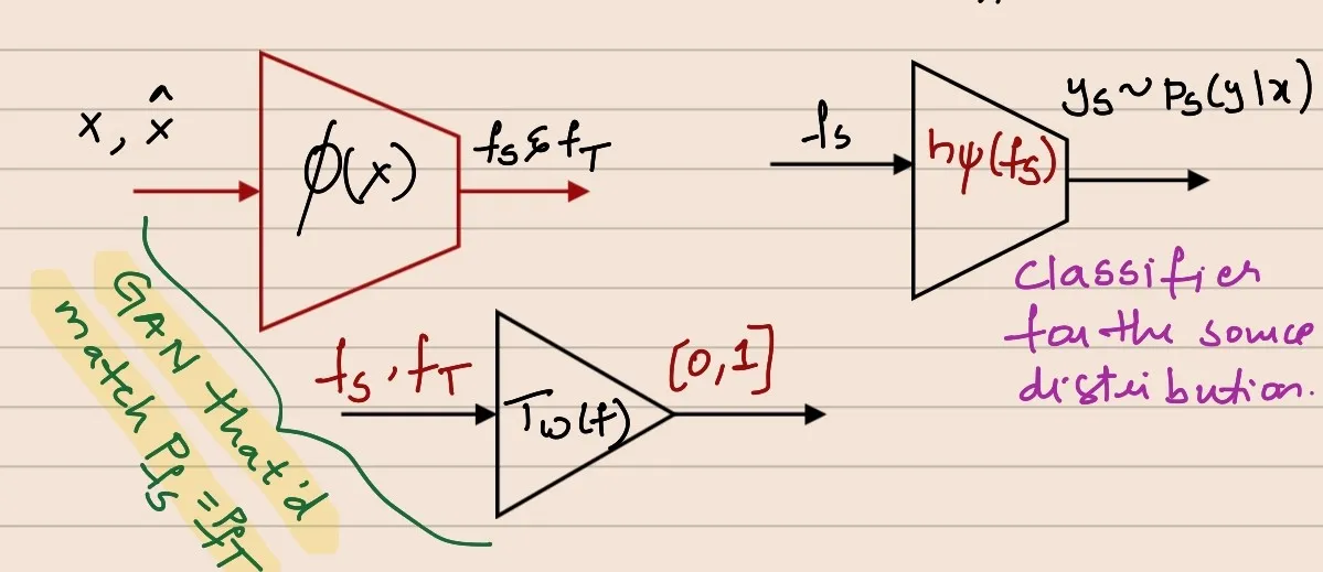
If we solely train the generator for the adversial objective, we may solve for the task of producing same representations for data points with same meaning well, but the produced representation may not be conducive for the classification task.

During inference, the same classifier can be used on both the source and target distributions, since the classifier is trained on domain-agnostic features.

Given,

Since $\phi$ would ensure that $P_{f_S} = P_{f_T}$, $h_{\psi^*}$ will function the same way irrespective of domain.

Implementation of UDA

Evaluation of Generative Models

Given $D_{\text{true}} = \{x_1, x_2, x_3, ..., x_n\} \mathop{\sim}^{\text{i.i.d}} P_x$ (Real Data), $D_{\text{gen}} = \{\hat{x_1}, \hat{x_2}, ..., \hat{x_n}\} \mathop{\sim}^{\text{i.i.d}} P_{\theta^*}$ (Generated Data)

**Goal: Compare $D_{\text{true}}$ & $D_{\text{gen}}$

A popular metric to do that comparison is Frechet Inception Distance

Frechet Inception Distance

FID: Wassertstein’s Metric between $D_{\text{true}}$ & $D_{\text{gen}}$ with a twist.

1. Take a pretrained inception net, trained on Image-Net.
2. Pass $D_{\text{true}}$ & $D_{\text{gen}}$ through the above inception network

Extract the features for $D_{\text{true}}$ & $D_{\text{gen}}$ from an $l^{\text{th}}$ layer of $I_{\psi^*}(x)$

3. Compute Mean and Co-Variances for $\hat{D}_{\text{gen}}$, $\hat{D}_{\text{true}}$

   $$\begin{gathered} \mu_{\text{true}} = \frac{1}{n} \sum_{i=1}^n Z_{\text{true}}^i \\ \Sigma_{\text{true}} = \frac{1}{n} \sum_{i=1}^n Z_{\text{true}}^i(Z_{\text{true}}^i)^T \end{gathered}$$

   Similarily, compute $\mu_{\text{gen}}$ & $\Sigma_{\text{gen}}$

4. Assume, $\begin{aligned} Z_{\text{true}} \sim N(\mu_{\text{true}}, \Sigma_{\text{true}}) \\ Z_{\text{gen}} \sim N(\mu_{\text{gen}}, \Sigma_{\text{gen}}) \end{aligned}$

5. FID = $W(N(\mu_{\text{true}}, \sigma_{\text{true}}) || N(\mu_{\text{gen}}, \sigma_{\text{gen}}))$ = $||\mu_{\text{true}} - \mu_{\text{gen}}||^2 + tr(\sigma_{\text{true}} + \sigma_{\text{gen}} - 2(\sigma_{\text{true}} \sigma_{\text{gen}})^{\frac{1}{2}})$

The Generative Model is better if FID is lower.

Lower FID ==> lower Wasserstein distance between $P_X$ and $P_{\theta^*}$

Reference Papers

1. GAN Paper: https://arxiv.org/pdf/1406.2661
2. f-GAN Paper: https://arxiv.org/pdf/1606.00709
3. Conditional GAN Paper: https://arxiv.org/pdf/1411.1784
4. DC-GAN Paper: https://arxiv.org/pdf/1511.06434
5. W-GAN Paper: https://arxiv.org/pdf/1701.07875
6. BiGAN Paper: https://arxiv.org/pdf/1605.09782